
The phrase “we sequenced the sample” describes perhaps a quarter of the work and almost none of the decisions. The instrument that reads the bases is the most automated and most reproducible part of a sequencing workflow. It runs unattended, reports its own quality metrics, and fails in obvious ways when it fails at all.
The parts that determine whether the result is trustworthy sit on either side of it. Before sequencing comes library preparation, an enzymatic and physical process that converts genomic DNA into a form the instrument can read, and which introduces most of the biases that later analysis has to work around. After sequencing comes a computational pipeline that aligns hundreds of millions of short fragments to a reference genome and decides, position by position, whether the differences it sees are real.
Key takeaways
- Library preparation converts DNA into fragments carrying instrument-readable ends, and it is where most systematic bias enters.
- Index sequences let many samples share one flow cell, at the cost of a specific failure mode where reads land in the wrong sample.
- Sequencing by synthesis reads clusters of identical molecules simultaneously, so any loss of synchrony within a cluster degrades quality along the read.
- Depth and breadth of coverage are independent, and a high average depth routinely hides regions with almost none.
- Most apparent variants in a raw call set are artefacts of alignment, amplification or chemistry rather than genuine differences.
Fragmenting DNA and Building a Library
Sequencing instruments cannot read a chromosome. They read short fragments with defined ends, and the first job of library preparation is to turn a genome into a population of such fragments, uniformly and without losing regions along the way.
Fragmentation happens either physically or enzymatically. Physical methods use focused acoustic energy to shear DNA, producing breaks that are close to random with respect to sequence. Enzymatic methods use nucleases or a transposase, and they are faster, require less input material and less equipment, but they show sequence preference: the enzyme cuts more readily at some motifs than others, which makes fragment ends non-random and subtly distorts coverage. Neither approach is universally correct, and the choice is usually driven by how much DNA is available.
Once fragmented, the ends must be made chemically compatible with the adapters that will be ligated on. Shearing leaves ragged ends with single-stranded overhangs, so a polymerase fills in recessed strands and an exonuclease chews back protruding ones, producing blunt ends. A single adenine is then added to each end, because the adapters carry a matching single thymine overhang, and this small complementarity dramatically reduces the rate at which fragments ligate to each other instead of to adapters.
Many workflows then amplify the library by PCR, which is where the most consequential bias appears. Regions that are extremely rich or extremely poor in guanine and cytosine amplify less efficiently than average ones, so they end up under-represented before the instrument has seen anything. PCR-free protocols avoid this entirely and are preferred whenever input DNA is plentiful, which for clinical samples it often is not.
Adapters, Indexes and Multiplexing
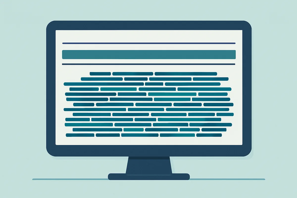
The adapter is a short synthetic double-stranded oligonucleotide with several distinct functional regions packed into it, and understanding those regions explains most of what happens on the instrument.
At the outer end sits a sequence complementary to oligonucleotides immobilised on the flow cell surface. This is what captures each fragment and holds it in place. Inboard of that lies a binding site for the sequencing primer, which defines where reading begins. Between them sits the index, a short barcode unique to the sample.
Indexing is what makes modern sequencing economical. A high-output instrument produces vastly more data than any single small sample requires, so many libraries are pooled and sequenced together, then separated computationally afterwards by reading their index sequences. This is multiplexing, and it turns an expensive run into an affordable per-sample cost.
It also creates a distinctive failure mode. Index hopping occurs when an index from one library becomes associated with a fragment from another, which can happen through free adapter molecules in the pool priming the wrong template, or through errors during cluster generation. The result is a small number of reads assigned to the wrong sample. For most applications this is negligible noise. For applications that hunt for rare variants at low frequency, such as detecting tumour DNA circulating in blood, hopped reads look exactly like the signal being sought. Unique dual indexing, where a different barcode sits at each end of the fragment and only expected combinations are accepted, is the standard mitigation.
Sequencing by Synthesis in Practice
The dominant chemistry reads DNA by building its complement one base at a time and photographing the result.
Library fragments are captured on the flow cell, and each one is amplified in place into a tight cluster of identical copies occupying a small patch of surface. The clustering step exists for a simple physical reason: the light emitted by a single molecule incorporating a single nucleotide is too faint to detect reliably, whereas a thousand identical molecules acting in unison produce a clear signal.
Each cycle then adds nucleotides carrying two modifications: a fluorescent label identifying the base, and a chemical group blocking the position where the next nucleotide would attach. Because that position is blocked, exactly one base is added per cycle regardless of what the template says next. The instrument washes away unincorporated nucleotides, images the flow cell to record which colour each cluster shows, then chemically removes both the label and the blocking group so the next cycle can proceed.
The consequences of this design are visible in every quality report. Because the cluster is read as a unit, every molecule in it must remain in step. Some do not: a molecule that fails to incorporate falls a base behind, and one whose blocking group was removed prematurely runs a base ahead. These errors are irreversible and cumulative, so the fraction of out-of-phase molecules grows with each cycle. The cluster’s signal becomes progressively blurred, and quality scores decline steadily along the read. This phasing behaviour, not any limitation of the enzyme, is the fundamental reason short-read sequencing is short.
Read Length and Why It Matters
Read length determines what a sequencing experiment can and cannot resolve, and no amount of extra data compensates for reads that are too short for the question.
The core difficulty is repetition. Genomes contain large quantities of repeated sequence: short tandem repeats, dispersed elements present in many thousands of copies, and segmental duplications spanning long stretches of near-identical sequence. A read that lies entirely within a repeat cannot be placed, because it matches many locations equally well. Aligners handle this by assigning a low mapping quality, which tells downstream tools to distrust the placement. Regions built largely from such sequence therefore return few confidently placed reads regardless of how much sequencing was performed.
| Approach | Typical read length | Strength | Main limitation |
|---|---|---|---|
| Short-read sequencing by synthesis | Hundreds of bases | High per-base accuracy, low cost per base | Cannot span repeats or large rearrangements |
| Long-read single-molecule sequencing | Tens of thousands of bases | Resolves repeats, structural variants and phasing | Higher per-base error, more input DNA, higher cost |
| Paired short reads | Hundreds of bases, known separation | Recovers some structural information cheaply | Inference is indirect and misses complex events |
| Linked or barcoded short reads | Short reads sharing a molecular tag | Long-range context at short-read accuracy | Additional preparation complexity |
Long-read technologies address these problems by sequencing single molecules across tens of thousands of bases, spanning entire repeats and rearrangements. Their historical weakness was per-base accuracy, which has improved substantially, and their remaining costs are financial and in the amount of intact high-molecular-weight DNA required. In practice many laboratories now use both, with short reads providing accurate base calls and long reads providing structure.
Coverage Depth Versus Breadth
Coverage is reported as a single average number and behaves nothing like one.
Depth at a position is simply how many reads overlap it. It matters because sequencing is a sampling process and calling a variant means distinguishing a real difference from a chance run of errors. For a heterozygous variant, roughly half the reads should carry the alternative base, and confidence in that ratio depends on how many reads there are. Detecting a variant present in only a small fraction of cells, as in a tumour sample or a mosaic condition, requires far more depth, because the signal must be separated from the background error rate of the chemistry itself.
Breadth is what fraction of the target region achieved some minimum depth, and it is the number that actually predicts whether a clinically relevant position was assessed. The two diverge because coverage is profoundly uneven. Regions with extreme base composition amplify and cluster poorly. Repetitive regions attract reads that cannot be confidently placed. Capture-based approaches, which use probes to pull down regions of interest, add their own unevenness because probe efficiency varies.
The result is that a report announcing a high average depth may conceal specific exons with almost none. A well-constructed report therefore states the proportion of target bases above a defined depth threshold and lists regions that fell below it, so that a negative result can be qualified honestly. A gene that was not adequately covered was not actually tested, and treating a negative call in such a region as a genuine absence is one of the more consequential errors in interpretation.
Alignment and Variant Calling Pipelines
The raw output is an enormous collection of short sequences with per-base quality estimates and no idea where they came from. Turning that into a variant list is a chain of computational steps, each of which can be tuned and each of which can go wrong.
Alignment places each read at its most likely origin in a reference genome. Because searching hundreds of millions of reads against a multi-billion-base reference exhaustively is infeasible, aligners use compressed index structures to find candidate locations rapidly, then perform detailed comparison only at those candidates. Each placement receives a mapping quality reflecting how much better the best location was than the alternatives, and this score, not the base qualities, is what governs trust in a read’s position.
Post-alignment processing follows. Duplicate reads arising from PCR amplification of the same original molecule are marked, because they represent one observation rather than several and would otherwise inflate apparent confidence. Base quality scores are frequently recalibrated against observed error patterns, since instrument-reported qualities are systematically biased by sequence context and cycle number. Regions around insertions and deletions may be locally realigned, because an aligner comparing a read to the reference independently will often represent the same indel in several inconsistent ways.
Variant calling then evaluates each position probabilistically. The caller considers the observed bases, their qualities, the mapping qualities of their reads, and a prior expectation about how often variants occur, and computes the likelihood of each possible genotype. Modern callers work on local haplotypes rather than single positions, reassembling the reads in a window into candidate sequences and asking which combination best explains the data, which handles clustered variants and indels far better than position-by-position analysis.
Filtering is the final and most opinionated stage. Calls are removed or flagged on the basis of depth, allele balance, strand distribution, position within reads, and proximity to other calls. Every filter trades sensitivity against specificity, and a pipeline tuned for research discovery and one tuned for clinical reporting will legitimately produce different output from identical input data.
Distinguishing Real Variants From Artefacts
A raw call set from a human genome contains millions of variants, and the overwhelming majority are ordinary population variation. Among the remainder, a substantial number are artefacts, and recognising their signatures is the core analytical skill.
Mapping artefacts are the largest class. When a read from a repeated region is placed at the wrong copy, every difference between the two copies appears as a variant. These calls cluster tightly, sit in regions of known duplication, and are accompanied by low mapping qualities and often by locally elevated coverage from reads piling in from elsewhere. A variant that appears only in a pseudogene-adjacent region and has never been seen in population databases despite being easy to call deserves immediate suspicion.
Chemistry artefacts have characteristic fingerprints. Oxidative damage during sample handling produces a specific base change that appears predominantly on one strand, so a variant supported almost entirely by reads in one orientation is suspect. Formalin fixation, used routinely for pathology specimens, causes deamination that produces another characteristic change, and this is the reason variant calls from archival tissue require different thresholds from those on fresh material. Homopolymer runs, stretches of a single repeated base, generate insertion and deletion errors at elevated rates in every chemistry.
The practical defences are consistent. Inspect the alignment visually rather than trusting the call: a genuine heterozygous variant shows a balanced allele ratio, support from reads in both orientations, and support from reads whose start positions vary. Compare against population frequency databases, since a variant common in the population is unlikely to explain a rare condition and a variant absent from every database in an easily sequenced region is more likely to be an error than a discovery. Confirm anything that will drive a decision by an independent method on an independent extraction, because that step catches sample mix-ups and contamination as well as calling errors.
The general lesson of the whole workflow is that sequencing produces evidence, not answers. The instrument reports what it observed with an honest estimate of its own uncertainty, and every subsequent step either preserves that honesty or quietly discards it. Reports that state coverage breadth alongside average depth, that name the regions which failed, and that separate confident calls from marginal ones are describing the same underlying data as reports that state only a headline number. The difference is that they let a reader know which parts of the genome were actually examined.
Frequently asked questions
Why does the same sample sometimes give different variant calls in two laboratories?
Because a variant call is the output of a long chain of choices rather than a direct observation. The two laboratories may fragment DNA differently, use capture probes with different efficiencies, sequence to different depths, use different aligners, and apply different filtering thresholds. Agreement is generally excellent for confidently covered positions with balanced allele support and poorer at the margins: low-coverage regions, repetitive sequence, indels in homopolymer runs and low-frequency somatic variants. This is why proficiency testing and reference materials with known genotypes are used to benchmark pipelines rather than assuming equivalence.
What does coverage depth of a given number actually guarantee?
Less than it appears, because the figure quoted is almost always an average across the target. Coverage is unevenly distributed by base composition, repeat content and capture efficiency, so a high average is entirely compatible with individual regions receiving very few reads. The meaningful metric is breadth: the fraction of target bases reaching a stated minimum depth, together with an explicit list of regions that did not. A negative result in an inadequately covered region is not evidence of absence, and reports that make this distinction are considerably more useful than those quoting a single number.
Why is library preparation described as the most important step?
Because it is the only step that can lose information irretrievably. Bias introduced during fragmentation, size selection or amplification determines which parts of the genome are represented in the pool, and no amount of downstream computation can recover a region that was never converted into a library molecule. Sequencing chemistry and analysis software have both improved markedly and are largely standardised; preparation remains hands-on, sensitive to input quality and quantity, and is where the differences between a clean dataset and a difficult one usually originate.
What are unique molecular identifiers for?
They are random sequences attached to each original DNA molecule before amplification, so that every read descended from the same starting molecule carries the same tag. This allows analysis software to group those reads and collapse them into a single consensus sequence, discarding differences that appeared during amplification or sequencing. The technique matters most when hunting variants present at very low frequency, such as tumour DNA circulating in blood, where a polymerase error copied into many reads would otherwise be indistinguishable from a genuine rare variant.
Do long reads make short reads obsolete?
Not currently, and the two are largely complementary. Long reads resolve what short reads structurally cannot: repeats, large rearrangements, and which variants sit together on the same chromosome copy. Short reads remain cheaper per base, need less intact high-molecular-weight DNA, and have a longer track record for accurate detection of single base changes. Many laboratories run both when the question warrants it, using long reads for structure and short reads for base-level accuracy, and the balance continues to shift as long-read accuracy improves.
This is education, not medical advice. Laboratory results only carry meaning alongside your symptoms, history and examination. Talk to a qualified clinician about your own results before changing anything about your care or supplements.